How AI Learns (Part 2): Deep Learning

Introduction

How is Artificial Intelligence getting so much smarter in such a short period of time? Recall that machine learning (ML) is a branch of AI that empowers computers to learn without being explicitly programmed. Deep learning is a sub-branch of ML based on multilayer neural networks, allowing computers to model complex patterns and data. In this article, we will dive into some core concepts and architectures of deep learning (a sub-branch of machine learning) that enable advanced learning by machines.

‍

Algo-r-(h)-i-(y)-thms, 2018 art installation. Source: Photo by Alina Grubnyak on Unsplash (accessed 08/21/2025)

Data in Deep Learning

Data is crucial in deep learning because it is used to train the models. We can distinguish data in multiple ways.

‍

Data can be segregated based on representation:

‍

• Numerical Data: Made up of integers or floating-point values that are measurable, countable, or additive. Can include time series data.
  
  • Discrete numerical values are countable and distinct, having a finite number of possible outcomes. For example, the number of defects in a product or the number of cars in a parking lot.
  • Continuous numerical values are measurable, with an infinite number of possible values within a range. For instance, temperature readings or race completion times.
• Categorical Data: Consists of labels or values that classify objects or individuals, with a specific set of possible values.
  
  • Nominal categories are without any inherent order. For example, car brands (Toyota, Tesla, BMW) or countries (United States, Japan, Spain).
  • Ordinal categories have a meaningful order, but lack a consistent numerical difference. For instance, customer satisfaction levels (Poor, Average, Good, Excellent) or education levels (High School, Bachelor’s, Master’s, Ph.D.).

‍

Data can be typed by structure: 

‍

• Structured Data: Referred to as quantitative data, it follows a predefined model or schema. To illustrate, flight reservations follow a rigid schema of reservation number, flight number, passenger name, etc.
• Unstructured Data: Also known as qualitative data, it doesn't have an internal structure. It can include text, video, and images. For instance, customer reviews and product photos can vary a lot and don't follow a rigid schema.
• Semi-structured Data: Falls somewhere in between structured and unstructured data. It lacks a predefined structure but uses metadata for definition. For example, JSON and XML objects have defined properties or tags.

‍

Data can be differentiated by the use of labels:

‍

• Labeled Data: Consists of input-output pairs. For instance, input images of cats with output labels of "cat" for image recognition.
• Unlabeled Data: No output labels provided. For example, market basket analysis to understand the sale of one product in relation to other products based on customer behavior.

Embeddings

Raw data is rarely used for the actual training. Conversion takes place to turn raw data into useful feature vectors, which contain the characteristics of the data points.

‍

Embedding is one encoding technique that works well for unstructured data and categorical data. It is a vector representation capturing semantic meaning. Embeddings can be compared to assess similarity and identify relationships.

‍

A diagram showing vector data. Source: Pinecone The Rise of Vector Data (accessed 08/21/2025)

Neural Networks Basics

You often hear "deep learning" and "neural network" together. They are related, but separate concepts. A neural network is a type of machine learning model, or architecture, inspired by the circuits of neurons in the human brain. You can visualize a neural network as a fully interconnected, directed graph structure organized by layers. A deep learning model is simply a neural network composed of more than three layers.

‍

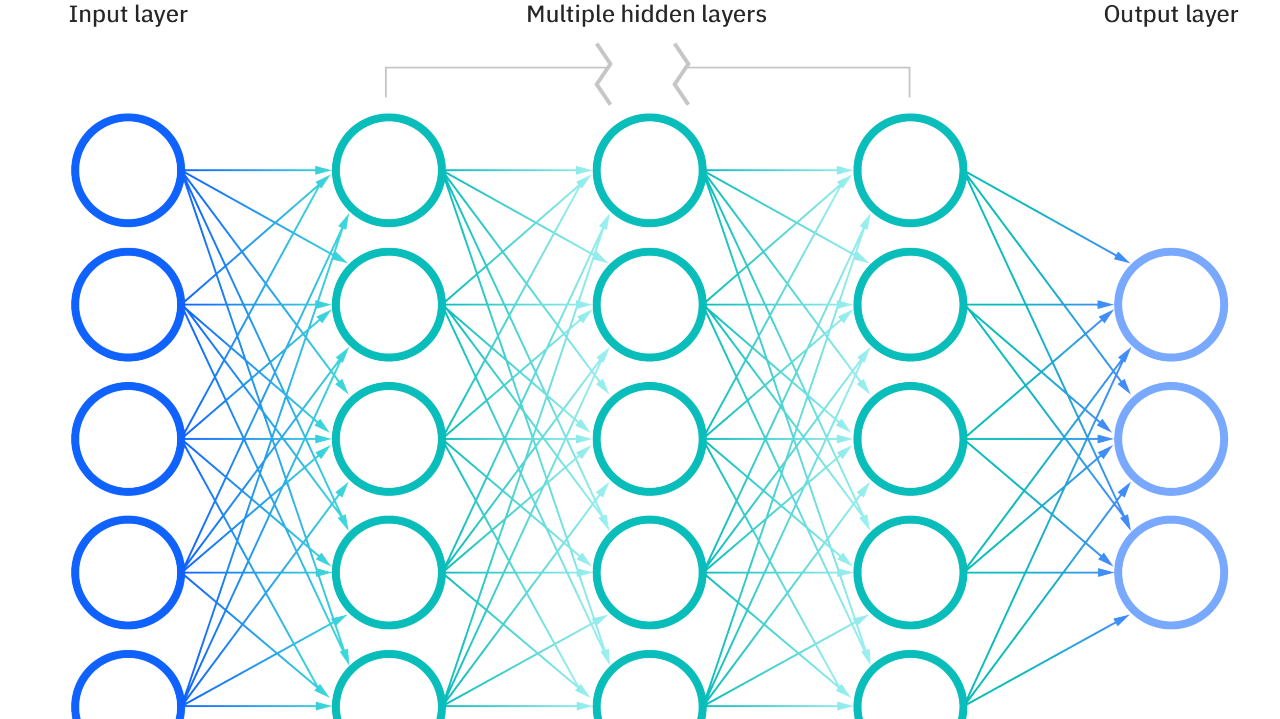
A visual representation of the layers in a neural network. Source: https://www.ibm.com/topics/neural-networks (accessed 08/21/2025)

The following are key components in a neural network:

• Node or Neuron: Each node or neuron is basically a function that takes in inputs and produces an output. An individual node may receive input from several connected nodes in the previous layer and may send output to several connected nodes in the next layer.
  
  • Weight: A node assigns a weight to each incoming connection to indicate how important that data source is. The node then computes the weighted sum of all inputs.
  • Threshold or Bias: The threshold value is a gatekeeper that determines whether the node passes its output to the next layer or not. Bias equates to the negative threshold and is added to the total weighted sum before it is passed through the activation function. 
  • Activation Function: A mathematical function that takes in the total weighted sum and bias to produce the node’s output. It decides how strongly a node should propagate through the rest of the network. Modern neural networks use a nonlinear function because complex, real-world problems are nonlinear.

A diagram of a neuron and its components. Source: https://www.codecademy.com/article/understanding-neural-networks-and-their-components (accessed 08/21/2025)

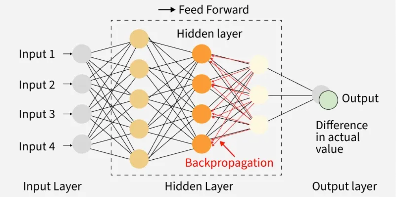
• Layers: There is 1 input layer and 1 output layer, which are known as visible layers. There are 1 or more hidden layers in between them.
• Directions:

A neural network diagram with feedforward and backpropagation. Source: https://www.geeksforgeeks.org/artificial-intelligence/artificial-neural-networks-and-its-applications/ (accessed 08/21/2025)

• Feedforward: Data moves from input layer to output layer until a decision is reached or output is produced. This is the progression of computations moving through the available layers of the network.
• Backpropagation: Data moves from output layer to input layer to calculate the error in prediction attributed to each node. The weights and biases are adjusted to improve output accuracy.

Initially, all of a neural network’s weights and biases are set to random values. As training data is successively fed through, the weights and biases are continuously adjusted automatically until the neural network produces expected outputs based on provided inputs. This process requires trial and error over time, similar to the human learning process.

‍

Neural Networks Optimization

Gradient Descent

The concept of gradient stems from mathematics, representing the rate and direction of change of a function. It is a vector pointing in the direction where the function decreases or increases most rapidly. In machine learning, the gradient indicates how to change model parameters to most efficiently decrease error or increase reward.

‍

Gradient descent is commonly used during backpropagation in deep learning models. It is a fundamental optimization algorithm to iteratively adjust the model's parameters (e.g., coefficients in linear regression or weights in a neural network) that result in the lowest possible error. A loss function is a mathematical formula that measures the difference (or error) between the predicted value and the actual value for a single data point. A cost function aggregates the loss values across the entire training dataset, resulting in a single overall measure of performance.

Hyperparameter Tuning

Hyperparameters are configuration settings that are set before model training. Unlike model parameters, which are learned from the training data, hyperparameters are defined externally to control different aspects of the learning process and model architecture.

‍

Some hyperparameters include:

‍

• Learning Rate: Controls the speed (or step size) that a model updates its parameters in each iteration. A higher rate means quicker learning, but increases the risk of suboptimal performance. On the other hand, a lower rate may improve performance, but requires more time and training data.
• Batch Size: Defines the number of training samples the model will compute before adjusting its parameters. A higher batch size can accelerate learning, but can weaken performance. In contrast, a lower batch size takes more time, but can improve performance and uses less memory.
• Epochs: Sets the number of times the model sees the entire training dataset. More epochs can improve performance, but overdoing it can lead to overfitting. This makes the model unable to generalize, reducing accuracy on new data.
• Number of Hidden Layers: Defines the depth of the neural network. More layers can improve performance, allowing for more complexity. However, it will be slower to train. On the contrary, fewer layers allow for a simpler and faster model, but can decrease accuracy.
• Number of Neurons or Nodes per Layer: Sets the width of the neural network. More neurons or nodes per layer increase the model's capacity to handle complexity among the data points. However, it will increase the training time required. Less width means a simpler and faster model, but can lower accuracy.
• Activation Function: Introduces nonlinearity into the neural network, enabling the network to learn complex patterns and relationships within the training data. Otherwise, the network is limited to performing simple linear transformations. Some common activation functions used in deep learning models are ReLU (Rectified Linear Unit), Sigmoid, Tanh (Hyperbolic Tangent), and Softmax.    
  
  • Activation Function Output Layer: Typically selected based on the type of prediction task. For binary classification, a Sigmoid or logistic function is suitable. For multiclass classification, Softmax is appropriate. For multilabel classification, Sigmoid is suited.
  • Activation Function Hidden Layers: Usually selected based on the type of neural network architecture. For instance, ReLU is used in Convolutional Neural Networks (CNNs). Tanh and/or Sigmoid are used in Recurrent Neural Networks (RNNs).

‍

The goal of hyperparameter tuning is to find the optimal combination of these hyperparameters that results in the best predictive accuracy, generalization, and efficiency of the deep learning model. Proper tuning reduces the issues of underfitting (inability to make accurate predictions) and overfitting (inability to generalize for new data). The tuning process can be computationally intensive, but it can enhance the model's overall performance (accuracy and consistency).

‍

Some hyperparameter tuning techniques include:

‍

• Grid Search: A brute-force approach that tries all possible combinations of defined discrete hyperparameter values to find the best combination. A simple, but computationally intensive technique, especially with a large number of hyperparameters. 
• Random Search: A sampling approach that randomly selects hyperparameter combinations based on defined statistical distributions for each hyperparameter. A more efficient technique than grid search. It works well when a few hyperparameters greatly impact the performance.
• Bayesian Optimization: A sequential approach that probabilistically selects the next best combination of hyperparameter values to try based on previous runs. It learns from the past to make smarter choices and is typically more efficient than grid or random search.

Deep Neural Networks

Convolutional Neural Networks (CNNs)

Introduced in 1989, Convolutional Neural Networks (CNNs) are inspired by the human visual system, excelling at classification and computer vision tasks (e.g., image classification and object detection). They can be computationally intensive, needing graphical processing units (GPUs) for training.  

‍

CNNs follow a multilayered architecture that increases in complexity. The earlier layers identify basic visual features, such as edges and colors. The latter layers focus on more complex, abstract visual concepts, such as shapes and objects.

‍

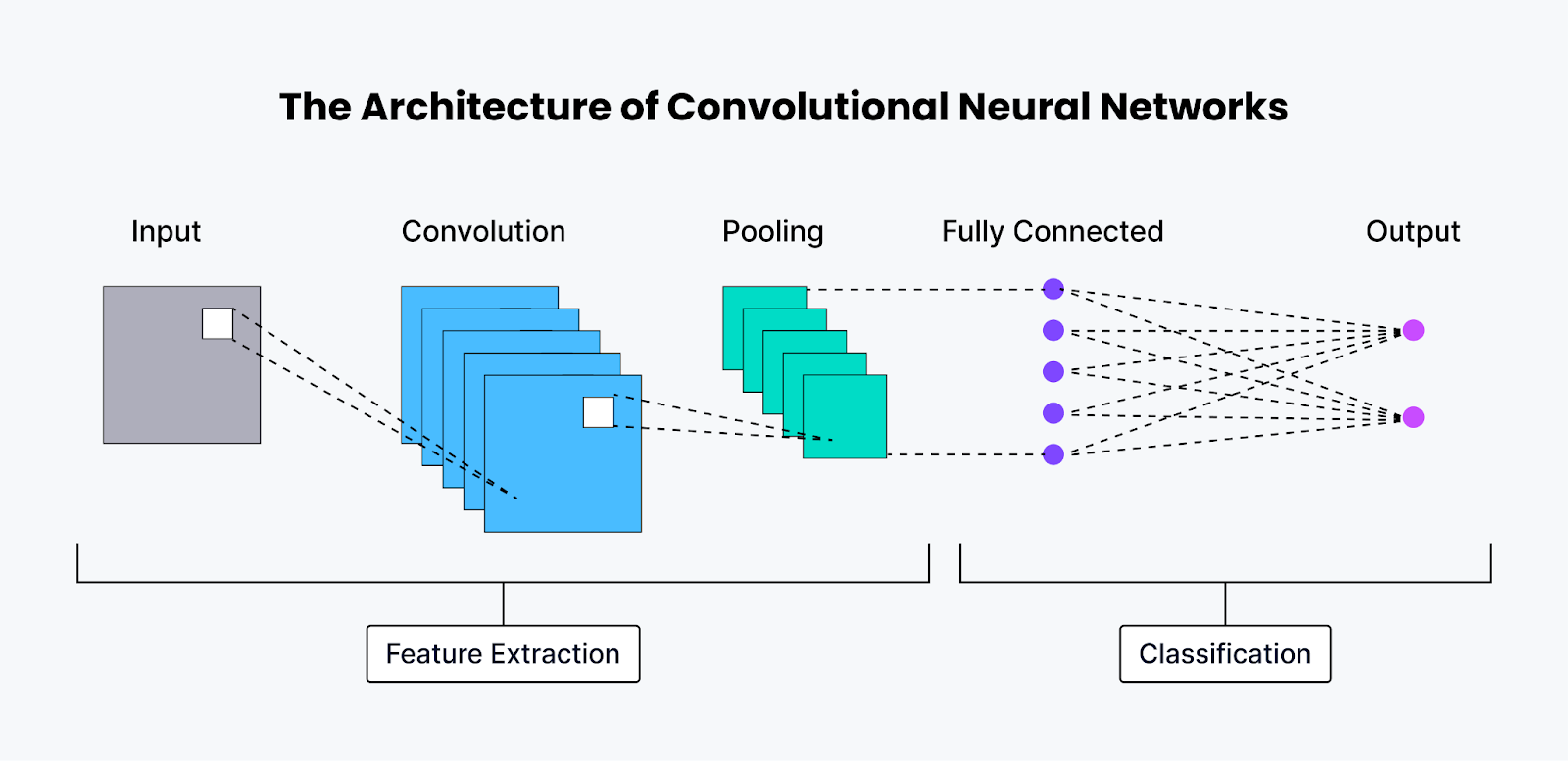
A diagram of CNN architecture. Source: https://zilliz.com/glossary/convolutional-neural-network (accessed 08/21/2025)

‍

Aside from the input and output layers, there are three main types of hidden layers (from earlier to latter):

‍

• Convolutional Layers: In each convolutional layer, a feature detector (or filter) sweeps across the image input data to check if a specific feature is present (e.g., edges, colors, or textures). An activation function, commonly ReLU, is applied after each convolution to introduce nonlinearity. This process repeats for each convolutional layer, eventually forming a feature map, which is a spatial outline of detected traits and patterns.
• Pooling Layers: The pooling layers perform dimensionality reduction on the incoming data, shrinking the spatial dimensions by only keeping the most relevant information. By simplifying, this improves efficiency and prevents overfitting. The following are some pooling methods:
  
  • Max Pooling: Takes the maximum value of each window in the feature map.

An illustration of max pooling. Source: https://www.geeksforgeeks.org/deep-learning/cnn-introduction-to-pooling-layer/ (accessed 08/21/2025)

‍

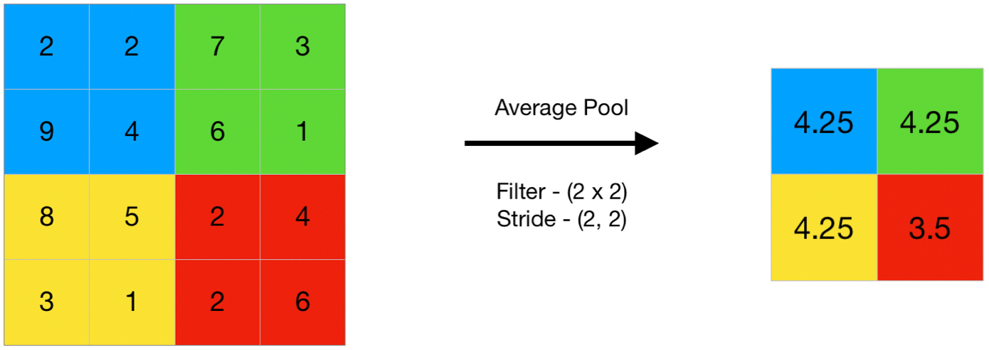
• Average Pooling: Takes the average of all the values of each window in the feature map.

An illustration of average pooling. Source: https://www.geeksforgeeks.org/deep-learning/cnn-introduction-to-pooling-layer/ (accessed 08/21/2025)

‍

• Fully-Connected (FC) Layers: The FC layers flatten the feature map before performing high-level analysis or classification. The Softmax activation function is commonly used for classification.

‍

CNNs allow for a more scalable approach to computer vision tasks due to automatic feature extraction, learning relevant visual features directly from the raw data. Previously, manual feature extraction methods were used for image classification and object recognition. CNNs lay the foundation for advances in object detection, facial recognition, video analysis, and medical imaging.

Recurrent Neural Networks (RNNs)

Introduced in the early 1980s, Recurrent Neural Networks (RNNs) are trained on sequential or time series data. Unlike traditional deep neural networks, which process input data independently, RNNs have a memory mechanism that remembers information from previous inputs. Hence, they suit tasks that deal with ordered data (e.g., natural language processing for language translation) or make sequential predictions (e.g., predicting rain levels based on past daily weather information).

‍

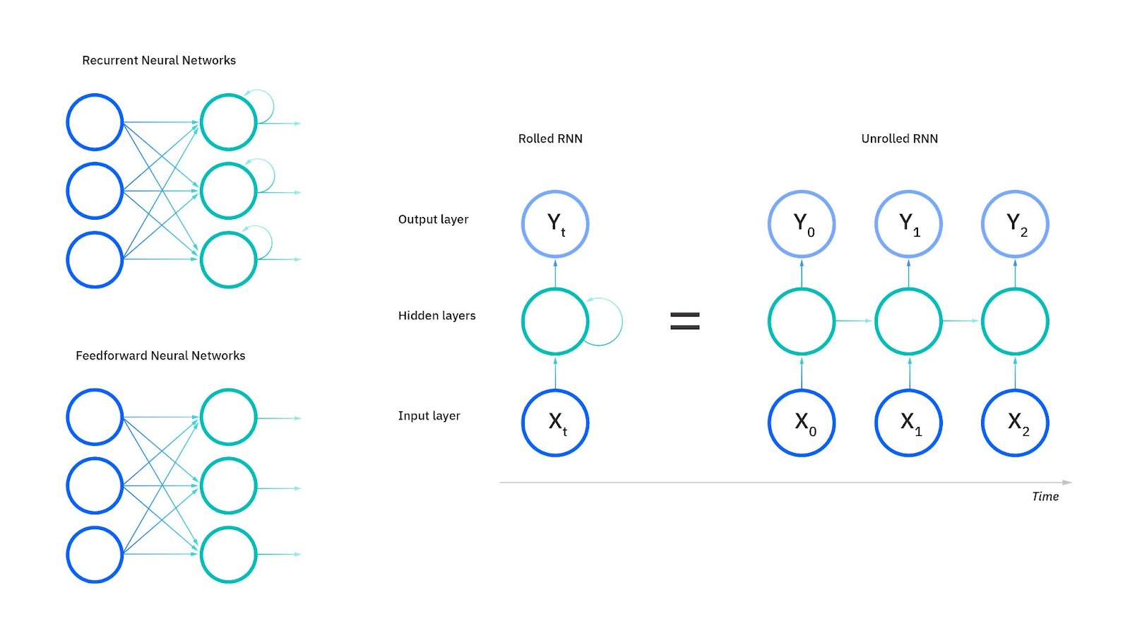
Recurrent Neural Networks vs. Feedforward Neural Networks. Source: https://www.ibm.com/think/topics/recurrent-neural-networks (accessed 08/21/2025)

‍

The following are the core layers:

‍

• Input Layer: Processes sequential data one step or element at a time.
• Recurrent Hidden Layers: Each node remembers historical knowledge by maintaining a hidden state, which is updated based on its prior value and the current input. 
• Output Layer: Uses the latest hidden state to predict, either after each step (e.g., language modeling) or full sequence (e.g., sentiment analysis).

‍

Unlike traditional deep neural networks, RNNs share the same weights among all nodes within each layer of the network. This allows for model efficiency, handling sequences of arbitrary length without escalating the number of weights that need to be learned. Additionally, this allows for consistency, as RNNs apply the same transformation to the input at each step.

‍

Due to the sequential nature, RNNs use Backpropagation Through Time (BPTT), an extension of the standard backpropagation. BPTT updates weights based on the current step and all prior steps, essentially unrolling the network over time. 

‍

There are multiple ways to configure RNNs: 

‍

• One-to-One: Processes a single input to produce a single output. Commonly seen in basic classification tasks, such as assigning an input image a label of "cat."
• One-to-Many: Channels a single input to multiple outputs. For example, using a keyword to generate a sentence for image captioning.
• Many-to-One: Takes multiple inputs and maps to a single output. For example, predicting the overall sentiment from several testimonials.
• Many-to-Many: Uses multiple inputs to predict multiple outputs. For instance, translating a sentence of several words from one language to another.

‍

However, RNNs are prone to exploding and vanishing gradient issues. Exploding gradient occurs when the gradient approaches infinity exponentially fast, causing the model to behave erratically such as overfitting. On the other hand, vanishing gradient happens when the gradient approaches zero exponentially fast, leaving the weights unadjusted and resulting in underfitting. Furthermore, training RNNs demands significant computational power, memory, and time due to the processing of sequential data in a serialized manner.

‍

These limitations have resulted in the decline of RNNs and the rise of transformers, which are parallelized and better capture long-range dependencies.

Transformers

Introduced in 2017, the transformer deep learning architecture enables processing of sequential input data in a non-serialized manner. Transformers combine the encoder-decoder setup with the concept of “self-attention.” This self-attention mechanism allows the entire input sequence to be processed simultaneously, increasing model efficiency with parallelization and capacity for understanding long-range dependencies.

‍

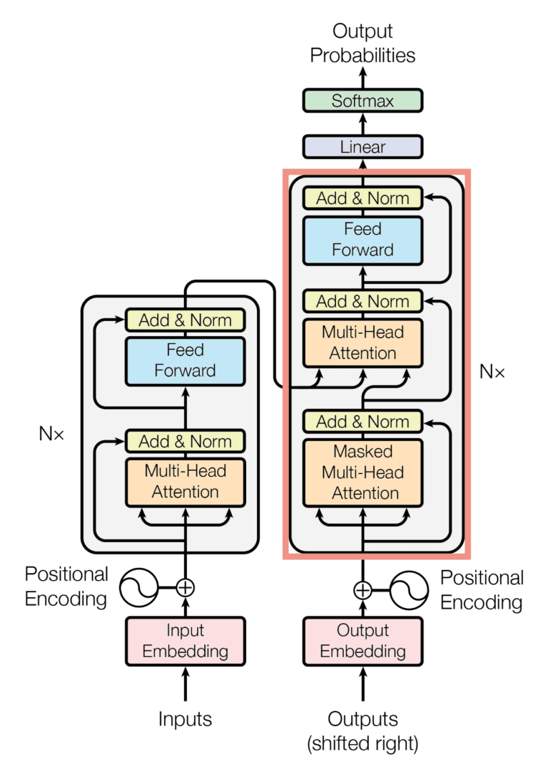
A diagram of the transformer architecture with encoder on the left and decoder on the right. Source: https://arxiv.org/abs/1706.03762 (accessed 08/21/2025)

‍

Here's an overview of the main blocks and layers:

‍

• Input Embedding Layer: Transforms each part of the input sequence into an embedding, which is a vector representation that captures the core meaning. Adds positional encodings to embeddings.
  
  • Positional Encoding: A representation of the order in which input parts occur. Since the entire input sequence is processed simultaneously, the transformer needs to preserve the order of the input parts in some way. Information indicating its position in the sequence is added to each part's embedding.
• Encoder Block: The encoder processes the entire input sequence. It is made up of several identical layers (e.g., 6), where each layer is composed of sublayers.
  
  • Self-Attention Sublayer: An attention weight is assigned to each part of an input to signify its importance in context with the rest of the input. The attention weights are derived from alignment scores, determined from comparing the embeddings, and then fed into a Softmax activation function. This self-attention mechanism enables the transformer to look at all the parts of the sequence simultaneously and decide which parts are the most important. Hence, the transformer can handle longer pieces of input text where context from the beginning might influence the meaning of words coming later.
  • Feed-Forward Network (FFN) Sublayer: Consists of two linear transformations and a ReLU activation function.
  • Normalization Sublayer: Ensures consistent scaling of activations.
  • Residual Connections: These skip connections allow information to bypass one or more layers, ensuring stable and efficient learning.
• Decoder Block: The decoder takes the encoder output, along with the previous decoder output, to generate the output sequence step by step. It is made up of several identical layers (e.g., 6), where each layer is composed of sublayers. Similar to the encoder block, common sublayers include feed-forward network (FFN), normalization, and residual connections.
  
  • Masked Self-Attention Sublayer: In contrast to the encoder block, the decoder block has an additional masked self-attention sublayer that processes the previous decoder output. The self-attention mechanism is modified here to attend to words preceding the current predicted word's position.

‍

Transformers overcome the gradient issues faced by RNNs with parallelization, avoiding the backpropagation limitations. Optimized for parallel computing, transformers can leverage the capability of graphic processing units (GPUs) to handle a massive amount of data and perform complex tasks.

‍

Transformers can be trained on different types of sequential data, such as human and programming languages, music, and even DNA sequences. However, transformers are most known for performing natural language processing (NLP) tasks, such as translation and summarization. There are also vision transformers (ViTs) that adapt the transformer architecture to process image data, which is not inherently sequential, with the workaround of patch embeddings.

‍

Summary

Deep neural networks allow computers to understand complex data and patterns. Through feedforward computation and backpropagation, these deep learning models automatically learn from the training data by continuously adjusting their weights and biases until they can accurately predict outputs from inputs. They also utilize activation functions to inject nonlinearity and better mimic complex, real-world scenarios. 

‍

Different deep learning architectures excel at specific tasks. Convolutional Neural Networks (CNNs) automatically extract visual features for computer vision tasks. Recurrent Neural Networks (RNNs) use a memory mechanism to process sequential data. Transformers utilize a self-attention mechanism to process an entire sequence simultaneously with parallel computing capability.

‍